Most of modern mathematics, and as a consequence, science at large assume the existence of real numbers, pretty much as a postulate¹. Given how successful both of these have been, it might seem odd to challenge it. However, when one takes a closer look at exactly how real numbers are defined, a couple of philosophical issues arise. In particular the fact that we (mere mortals) can only meaningfully interact with countably many of them, so that almost all real numbers are beyond our grasp. The goal of this post is to articulate this problem in a mostly self-contained and accessible manner, by constructing the real numbers from the ground up, and then discussing some philosophical consequences of the previously stated fact.

Much of the material in this post comes from Stillwell’s book on Reverse Mathematics², which is a delightful read I heartily recommend to anyone interested in logic and the foundations of mathematics.

Philosophical Hazards

This post touches on issues that were at the heart of the crisis of foundations of mathematics roughly a century ago, and created a schism among mathematicians at the time. Depending on your constitution, you may experience the following symptoms

• Indifference,
• Mild interest,
• Five stages of grief,
• Intuitionism and/or Constructivism.

I hope at least to elicit the second of these symptoms, but beware that the last two are only partially jokes. For your safety (and brevity), some technical details are omitted. Links to relevant background are included liberally in the text.

The Peano Axioms

God invented the integers. All the rest is the work of man.

— L. Kronecker

In order to make $\pi$ from scratch, we first have to invent the universe, which in our case means the basic language from which everything is built up. Namely, Peano arithmetic, which is the canonical formalization of the natural numbers. The rules of Peano arithmetic are essentially expressed in four axioms:

1. $0$ is a natural number.
2. If $n$ is a natural number, then its successor $S(n)$ (morally, ‘$n+1$’) is a natural number.
3. For all $n$, $S(n) \neq 0$, i.e. there is no natural number “before” $0$.
4. For all natural numbers $m, n$, $S(m) = S(n) \Rightarrow m = n$, i.e. the successor operation is injective.

In the above, I implicitly assumed the existence of an equivalence relation ‘$=$’ between natural numbers, as well as the usual predicate logic machinery (as indicated by the ‘For all’). The last important axiom of Peano arithmetic is the axiom of induction, which declares that we are allowed to do proofs by induction:

where $\varphi$ is a unary predicate. In the “standard” model of arithmetic based on set theory, we can then form what we know as the set of natural numbers

Of course, the Peano axioms are just axioms, i.e. an abstract “interface”, which we may implement in various ways. For example, we can implement them in set theory by defining $0$ to be the empty set $\emptyset$, and the successor operation to be \(S(n) = n \cup \{n\}.\)

The first few natural numbers then look like

Actually, we don’t even need to bother with the ‘$\emptyset$’ symbol, do we? We could just as well use an empty pair of braces {} :

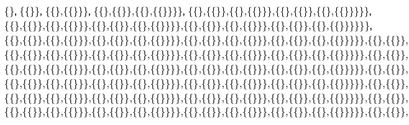
Jokes aside, this exemplifies the mindset of trying to axiomatize something in a formal language: Finding the absolute minimum amount of principles and syntax needed to define it.

Before moving on to the next section, we still need to define some arithmetic operations and relations on natural numbers. These are defined recursively.

• Order relation: $0 < S(n)$; $S(m) < S(n) \Leftrightarrow m < n$.
• Addition: $m + 0 := m$; $m + S(n) := S(m+n)$.
• Multiplication: $m\ast 0 := 0$; $m\ast S(n) := (m\ast n) + m$.

It is tedious, but relatively straightforward to show that addition is associative, commutative and has $0$ as an identity element, that is, that $(\mathbb{N}, +, 0)$ is a commutative monoid, and that multiplication is associative, commutative and distributive with addition.

Integers

So far, we’ve constructed the natural numbers, which lack the notion of additive inverse to form a group. There is a simple trick to construct a group from a monoid, which consists of taking pairs of monoid elements. In our case, we will define the set of integers as

where each pair $(m,n)$ should be interpreted as ‘$m-n$’. To wrap your head around this, it is helpful to think of fractions (it’s exactly the same idea). Let us also notice that any integer admits an infinite number of representations, much like rational numbers can be represented by different fractions. We also have a canonical injection of $\mathbb{N}$ into $\mathbb{Z}$ given by $ n \mapsto (n,0)$.

We need to extend our arithmetical operations on $\mathbb{Z}$:

These operations inherit the properties of the ones defined on natural numbers, so that with the addition of additive inverses, $(\mathbb{Z}, +, \ast)$ is now a ring.

Rational Numbers

From the previous section, the way to construct the rational numbers is straightforward. We simply take pairs of integers to form fractions, with the added constraint that the denominator must be positive:

That last constraint needs some additional care to preserve, but otherwise extending the operations is uncomplicated

With the addition of multiplicative inverses, $\mathbb{Q}$ is now a field.

Dedekind cuts

Now comes the tricky bit of actually defining real numbers. There are various ways to do that, but the canonical way is via Dedekind cuts. Formally, a Dedekind cut is a partition of $\mathbb{Q}$ into two sets $L$ and $U$ such that

• $L$ has no greatest element,
• $U$ has no smallest element,
• $\forall x \in L, y \in U, x < y$.

Morally, we are sorting all the rational numbers on a line, and cutting at some point to separate $\mathbb{Q}$ into a lower part $L$ and an upper part $U$. Because $L$ has no greatest element, and $U$ has no smallest element, there is an “infinitesimal gap” between $L$ and $U$, which corresponds to a unique real number.

After massaging this a bit, we finally arrive at our definition of real numbers:

A real number is a set $L \subset \mathbb{Q}$ with an upper bound, and such that if $s\in L$ and $t<s$, then $t\in L$.

For example, we can define the square root of $2$ as

More generally, any definition of a real number can be reduced to the form

where $\varphi$ is a unary predicate on $\mathbb{Q}$. This will be important later, as we will be restricting the class of predicates that can be used to define a real number.

Note that in this definition, we now allow $L$ to have a greatest element. This allows us to include the rationals with a canonical injection given by \(q \mapsto \{ p \in \mathbb{Q} \,|\, p \le q\}.\)

Due to real numbers being sets, the equality and order relations are easily defined as set equality and set inclusion:

Arithmetical operations do require a bit more care, though

The tricky part is defining multiplication. Simply taking the set of products of elements of $L_1$ and $L_2$ will not work, because $L_1$ and $L_2$ both contain unbounded negative numbers, whose products are unbounded positive numbers. To resolve this, we first define a new “signed” product on $\mathbb{Q}$

It is not too complicated to show³ that if $x,y \in \mathbb{R}$ and $p,q \in \mathbb{Q}$ such that $p \le x$ and $q \le y$, then $p \circledast q \le x \ast y$, so that we may define the product of two real numbers as

To recap a bit, we’ve just constructed real numbers as sets of rational numbers, which are just pairs of integers, which themselves are just pairs of natural numbers. Since $\mathbb{Q}$ is countable, there is a bijection between $\mathbb{Q}$ and $\mathbb{N}$, so that real numbers can be equivalently expressed as sets of natural numbers, and any real number can be defined in the following form

where $\varphi$ is a formula in some formal language containing the Peano axioms. Each real number therefore corresponds to a unique set of natural numbers (which depends on the encoding, i.e. the bijection $\mathbb{Q} \rightarrow \mathbb{N}$). Notice that we said a formula in some formal language. This is actually a very important detail. Different languages will be able to define different real numbers.

Turing machines and computable numbers

As an example of a formal language containing Peano arithmetic, let us look at computable numbers. These correspond to the numbers that can be calculated by a Turing machine. We don’t need to go over the definition of Turing machines here however, as they are the theoretical model of computers, so for the purposes of this post, computable number means a number that can be approximated by a computer.

More exactly, a real number $x$ is computable if its decimal expansion can be computed to an arbitrary precision using a Turing machine, or equivalently

• There exists a computable function that, given $\varepsilon >0$, produces a rational $q \in \mathbb{Q}$ such that $\vert x-q \vert <\varepsilon$.
• There exists a computable function that, given $n\in \mathbb{N}$ as input, produces the $n$-th digit in the decimal (or binary or any other base) expansion of $x$.
• The characteristic function of the Dedekind cut of $x$ is computable.

Algebraically, computable numbers form a field that contains

• rational numbers (trivially),
• algebraic numbers (i.e. roots of polynomials with integer/rational coefficients, using Newton’s method for example),
• some transcendental numbers like $\pi$ and $e$,
• computable functions ($\sin$, $\cos$, $\exp$, …) of computable numbers.

In fact, computable numbers contain most numbers we encounter in practice. However, computable numbers are countable!

Why? The reason is simple. A computable number has to be uniquely identified by a Turing machine (morally, a program), which takes up finitely many symbols chosen from a finite alphabet to express. This means the set of all programs/Turing machines is countable, so the programs that compute numbers must be countable too.

But since real numbers are uncountable, there must exist real numbers that are not computable.

Science is computable

While the previous remark may seem abstract, it actually has a direct impact on real life. Indeed, consider for a moment the numbers manipulated in scientific research. Where do they come from? There are essentially two options:

• Empirical measurements, which are necessarily of finite precision, hence computable,
• Calculations, either by hand or by computer, which are also computable, by definition.

Non-computable numbers can’t be measured or observed directly. They can’t be numerically approximated, and even if you somehow had one, you wouldn’t be able to communicate it to someone else. In other words, they are completely outside the grasp of the scientific method. Science can only deal with computable numbers.

It’s worth spending a moment to reflect upon this. If the scientific process is inherently computable, then by assuming the existence of all real numbers, we are admitting the existence of objects beyond science’s ability to prove. No scientific experiment will ever let us conclude that non-computable numbers exist. As a result, this may also mean that there are facts about the universe that science cannot prove.

Algorithmic complexity and randomness

Any one who considers arithmetical methods of producing random digits is, of course, living in a state of sin.

— J. Von Neumann

If science can only deal with computable numbers, why do we need the rest of real numbers? We can begin to answer that question by getting some intuition on these non-computable numbers, by using the notion of algorithmic complexity.

Formally, the Kolmogorov complexity $K_A(s)$ of a finite string of symbols $s=(s_1,\dots,s_n)$ in a given language⁴ $A$ is the length of the shortest program in $A$ that computes $s$.

Intuitively, Kolmogorov complexity captures the idea that some strings can be computed by very short programs. Another way to think about it is that certain strings are inherently “compressible”, since we’re essentially trying to compress strings into shorter descriptions, in exactly the same way a compression algorithm tries to condense a file in a smaller form.

For example, a string of alternating ‘0’s and ‘1’s could be computed in many programming languages as ‘"01" * 8’, which is shorter than writing "0101010101010101". For some strings, like "11001001011101001" however, there isn’t such an obvious way to express using a program, so that we are doing about as well as simply writing the whole string in the program. Note that we can always do that for any string, so that the length of the shortest program that produces a string is always at most the length of that string (plus some constant).

Now for an infinite string of symbols, we can look at how the Kolmogorov complexity of its finite prefixes evolves. Based on the examples in the previous paragraphs, we can expect two main cases. Either the string is simple enough that there is a single program that can generate all its prefixes and the Kolmogorov complexity remains bounded, or there isn’t and Kolmogorov complexity diverges to infinity.

Using this notion, we can define an algorithmically random number as a real number such that the Kolmogorov complexity of its truncated binary expansions $s$ satisfies \(K_A(s) > |s| - O(1),\) where $|s|$ denotes the length of the finite string $s$. In other words, the prefixes of $s$ are all “maximally complex”, and their Kolmogorov complexity diverges.

Algorithmically random numbers capture the idea of “random” numbers due to an important characterization: They are indistinguishable from random noise by any statistical test⁵. Another (which is really the same), is that there is no computable betting strategy that reliably makes money against the sequence of digits of an algorithmically random number.

Other important properties are that ARNs are not computable by definition, since if they were, their Kolmogorov complexity would not diverge. By the definition of Kolmogorov complexity, they are also fundamentally “incompressible”.

Thanks to these facts, we can now give an interpretation to non-computable numbers. They correspond to the intuitive notion of randomness. (This is in fact precisely what algorithmic randomness is meant to formalize).

Philosophical ramblings

Whereof one cannot speak, thereof one must be silent.

— L. Wittgenstein

After all this math, we should probably stop and look back on what it might all mean in practice. We looked at computable numbers and observed that they were pretty much the only numbers we encounter, and that non-computable numbers (which are actually almost all real numbers) fit our intuition of randomness. We can go further than that and explore what exists in mathematics beyond computable numbers, and do some armchair philosophy about how to interpret this formalized notion of randomness.

What does it mean to “know” a number?

In defining real numbers, I alluded to the idea that different formal languages (morally, sets of axioms) would be able to define different real numbers. For example, computable numbers are precisely the real numbers definable using only computable formulas.

Intuitively, to define a number means to be able to identify it uniquely using a finite description. In other words, it means we have a name for it. There are different kinds of names, and these kinds are of varying usefulness. For example, rational numbers are easier to understand and work with than Turing machines that compute real numbers.

More generally, a real number is said to be definable in a given formal language if it can be defined using a formula from that language. There is an entire zoo of classes of definable numbers beyond computable ones. The diagram below shows a small sample of the most recognizable ones.

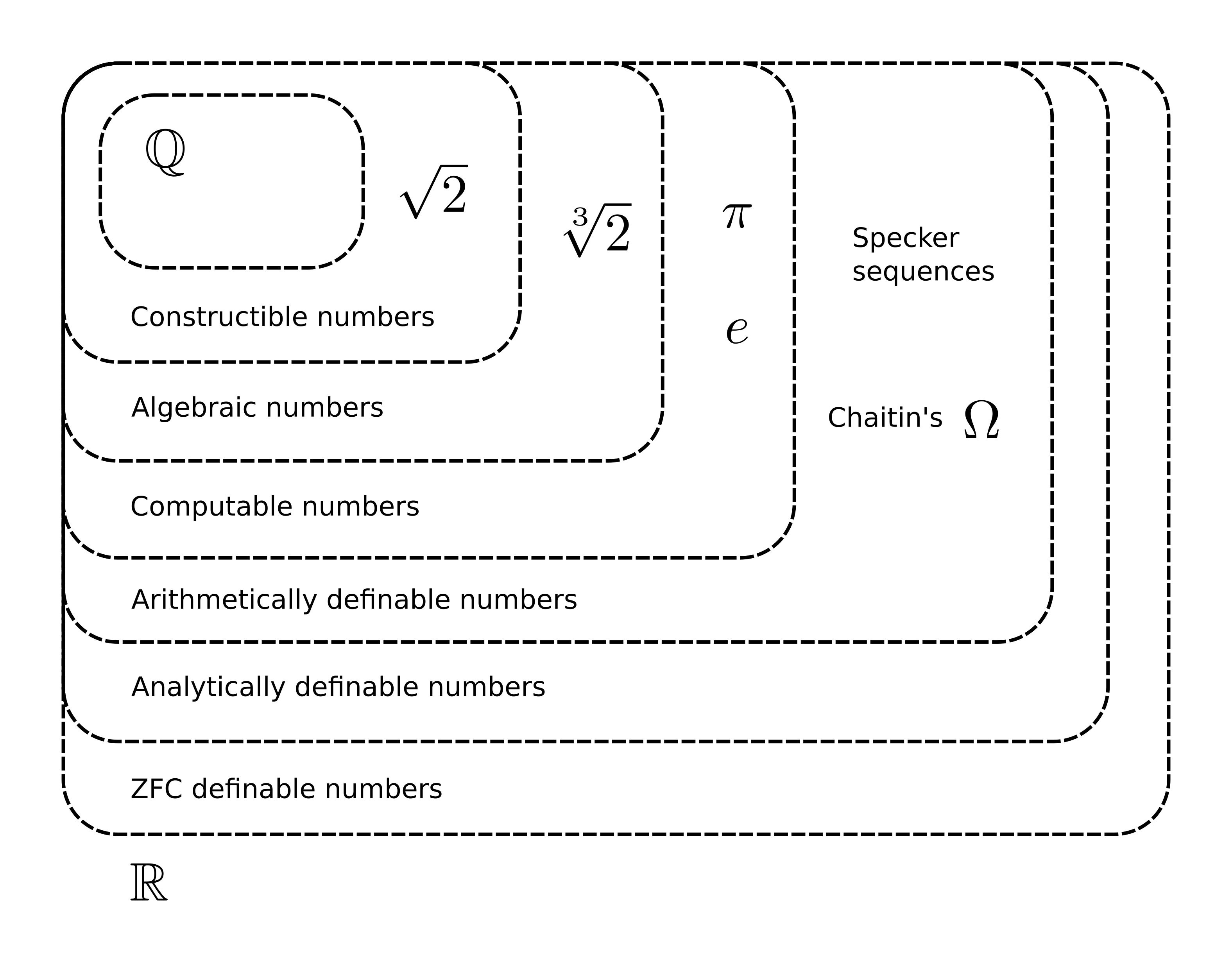
No matter which language we use, however, we will always suffer from the same flaw. Formulas in a formal language can only take finitely many symbols from a finite alphabet, and so they will always be countable. We will therefore only ever be able to define countably many real numbers, because we don’t have enough names for them.

Coming back to computable numbers, while there are numbers definable beyond them, such as those definable in first order arithmetic, the few examples that we have are rather esoteric and extremely cursed. They certainly don’t seem to correspond to any “nice” numbers that we might want to use to describe the real world. As such, it seems preferable to stick with computable numbers as those that best capture the intuitive notion of real numbers⁶.

The map, the territory, and the mapmaker’s mind

Let us conclude by continuing the discussion we started when observing that science can only manipulate computable numbers. If we think of science as the rational description of the empirical world, we can consider the following “picture”:

• The Territory, i.e. the (empirical) Universe⁷,
• The Map, i.e. Science,
• The Mapmaker, i.e. (Human?) minds.

As previously established, Science is computable, which leaves open the status of the other two parts. These are major philosophical questions that have never been more relevant than today.

First, whether human minds are computable. This is the founding postulate of the search for Artificial General Intelligence, arguably the holy grail of the field of computer science. This question has long been (and continues to be) the subject of vigorous debates, and I will not discuss it. I will simply note that personally, there seems to be little evidence for human minds being fundamentally non-computable, and plenty to the contrary.

There is another question that interests me more, however. If human cognition is computable, then how come we are able to conceive of non-computable things? What happens inside a mathematician’s mind when he/she thinks of say, Chaitin’s Omega? The straightforward answer would be that we are just fooling ourselves, but we seem to be able to reason perfectly fine about these objects supposedly beyond our comprehension.

Second, whether the Universe is computable. This could be otherwise stated as whether there is such a thing as true randomness. The obvious candidate for this would be quantum mechanics. As a side note, let us remark that probability theory, the usual way to deal mathematically with randomness, was initially created to deal with uncertainty, in the sense of things that we could in principle know, but don’t. The existence of “true” randomness would imply that there are things that we cannot know.

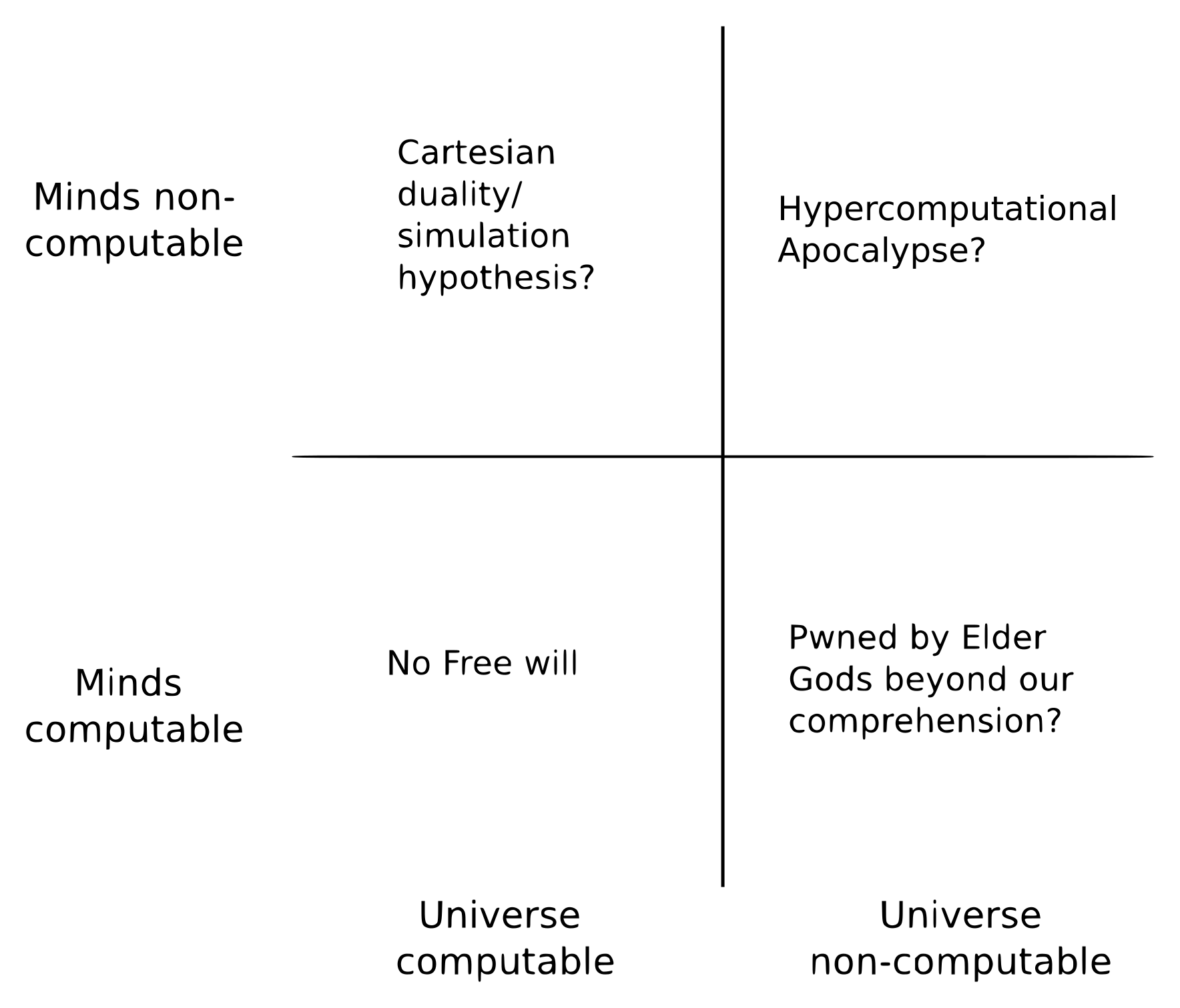
Finally, we can consider the combinations of these two questions:

1. If minds are non-computable, and the universe isn’t, then there must be clearly be something “outside” the empirical world from where our non-computable minds emanate. This would suggest something like Cartesian Dualism, or the Simulation Hypothesis.
2. If neither minds nor the universe are computable, there doesn’t seem to be much that we can say a priori, beyond the observation that there would be facts about the universe that science can never elucidate. There is however a wild possibility in that case⁸. If non-computable physical processes exist, it may be possible for us to harness them to perform hypercomputation. The consequences of that would be literally apocalyptic⁹, as we would be able to do things like solve the Halting Problem or solve the Collatz Conjecture by brute force in an instant. Since these would still be out of the grasp of computable science, we may have to develop a higher order “Hyperscience” that can cope with non-computable objects.
3. If both minds and the universe are computable, we seem to be in the opposite situation that science could in principle come to a complete description of the universe, but that since minds are computational processes (and therefore deterministic), the notion of Free Will is completely illusory.
4. If minds are computable, but the universe isn’t, we seem even worse off than in the previous case. Not only is Free Will an illusion (perhaps due to non-computable processes acting as inputs to our minds), but we have no hope of achieving a complete rational picture of the universe. Even worse, there might exist true non-computable minds, to which we would be as ants. This is probably not a good universe for us to exist in.

Conclusions and further reading

Hopefully, if you’ve read all the way until this point, you should probably agree that accepting real numbers as we commonly do is not as straightforward a philosophical position as it might have seemed, and that bringing in the full power of non-computable numbers also brings with it some rather counterintuitive things that don’t seem to physically make sense.

Where do we go from here? One reaction would be to reject non-computable mathematics entirely and become a constructivist. While I mentioned that computable numbers are not necessarily nice to work with, there is nonetheless a large body of beautiful mathematics, built around examining the intricate relations between theorems from classical mathematics and the formal languages that can prove them (possibly in a weaker form). Some go all the way into exploring parallel mathematical universes.

If you think Intuitionism is a bit too restrictive, see Predicativism[^predicative], which posits that one can only define a set if all it’s elements are already “accessible”. One practical consequence of this is that we cannot form infinite power sets, so that the set of real numbers cannot be constructed, but can be “approximated” by a hierarchy of countable sets.

From the physics side, see the recent work by Nicolas Gisin, who has been arguing that physics should reject classical logic (and non-computable numbers) and embrace intuitionism.