The Julia programming language currently holds the state of the art in terms of ODE solvers, and comes with a variety of ways of specifying ODEs. A common use case is to define modular dynamical systems, where the same pieces occur in multiple places with a bit of variation. Examples of this include running multiple copies of the same system with different parameters for each copy, or dynamical systems on networks like reaction-diffusion systems.

In this post, I’ll cover three different ways of specifying such systems using various packages from the Julia ecosystem. In particular, I’ll discuss some of the gotchas of each method. I’ll conclude by comparing the performance of the each approach.

All the code shown in this post can be found here. At the time of writing, I was using Julia 1.9.0 with DifferentialEquations v7.7.0, ModelingToolkit v8.56.0 and NetworkDynamics v0.8.1.

Thanks to Sundar R, Michael Lindner and Frank Hellmann, who provided helpful comments on the Julia Slack and Github.

Background: Reaction-Diffusion systems on networks

As the main example throughout this post, we’ll be modeling generic dynamical systems on networks. Those are typically of the form

where $f$ is a function describing the local dynamics at node $i$, $A$ is the adjacency matrix of some graph with $N$ nodes and $g$ is a function describing the pairwise dynamics on two nodes connected by an edge. The classical choice for $g$ is to take $g(x_i,x_j) = x_j - x_i$, which leads to the Laplacian coupling (also known as diffusion coupling). The parameter $D$ is a constant describing the rate of diffusion.

For our demonstration, we will use the famous Brusselator model for the local dynamics. It consists of two equations given by

where $a$ and $b$ are parameters of the model. The Brusselator model originally comes from chemical reactions, and when running multiple copies of it coupled by the edges of a graph with the Laplacian coupling, we call this a network reaction-diffusion system.

When using the Brusselator dynamics in a network reaction-diffusion system, we’ll equip each node $i$ of a graph with variables $u_i$, $v_i$, subject to the equations

If we allow borrowing some notations from Julia, we can rewrite these in vector form as

where $f_u(x,y) = a + x^2 y - bx - x$, $f_v(x,y) = bx - x^2 y$, and the ‘.’ indicates elementwise evaluation, or broadcast as it’s known in Julia. The matrix $L$ is the Laplacian matrix $D-A$ of the graph, where $A$ is the adjacency matrix, and $D$ is a diagonal matrix whose entries correspond to the degrees of the graph’s nodes ($D_{ii} = \sum_j A_{ij}$). This last form of the equations is the most concise, and the most handy for us as it involves operations we can easily express in Julia, namely broadcasting and matrix-vector multiplication.

Approach 1: Manually defining the ODE function

The first method, which is the one I usually use, is simply to manually define the ODE function for my problem. Let’s start by defining some functions for the Brusselator dynamics that will come in handy throughout this post.

brusselator_x(x,y,a,b) = a + x^2 * y - b*x - x
brusselator_y(x,y,a,b) = b*x - x^2 * y

Now, the proper way to define dynamical systems in Julia this way is to use in-place function to avoid allocating memory. Let’s do that now.

function brusselator!(dx, x, p, t)
    # a, b = p
    dx[1] = brusselator_x(x[1], x[2], p[1], p[2])
    dx[2] = brusselator_y(x[1], x[2], p[1], p[2])
end

We can use this function to simulate the base Brusselator model, but we’d like to use it in a networked system. Now, at that point we have to think about something. For our networked system, we need to stack $N$ copies of the basic system into a single array, but there are two ways we could do that: either as a $2 \times N$ or $N \times 2$ array. This is important because Julia stores arrays in Column-Major-Order, so it’s always more efficient to do operations column-wise rather than row-wise. In this case, we expect the matrix multiplication to dominate the cost as $N$ gets large, so we’d like to have the inputs of our matmuls within columns. Therefore, using an $N \times 2$ array is the best choice in this case.

Let’s write an in-place function for our reaction-diffusion system using the brusselator! function then. A simple implementation might look like

function brusselator_rd_1!(du, u, p, t)
    a, b, L, D = p
    for i in axes(du, 1)
        brusselator!(view(du, i,:), view(u, i,:), [a, b], t)
    end
    du[:,1] .-= D[1]*L*u[:,1]
    du[:,2] .-= D[2]*L*u[:,2]
end

which is decent enough, but the matrix-vector multiplication L*u[:,1] allocates memory, which we want to avoid. Let’s replace it with the in-place mul! function.

function brusselator_rd_2!(du, u, p, t)
    a, b, L, D = p
    for i in axes(du, 1)
        brusselator!(view(du, i,:), view(u, i,:), [a, b], t)
    end
    mul!(view(du,:,1), L, view(u,:,1), -D[1], 0.0) # du[:,1] .-= D[1]*L*u[:,1]
    mul!(view(du,:,2), L, view(u,:,2), -D[2], 0.0)
end

Notice the use of view when calling in-place functions like brusselator! or mul!. This is important, as calling view creates a view of our array, which means du will correctly be updated by our in-place functions. This is not the case if we just index into the array with e.g. u[:,1].

Having to write view(...) everywhere in our code gets tedious fast though, so luckily we can use the @views macro to make everything cleaner.

function brusselator_rd!(du, u, p, t)
    p_b, L, D = p
    @views for i in axes(du, 1)
        brusselator!(du[i,:], u[i,:], p_b, t)
    end
    @views begin
        mul!(du[:,1], L, u[:,1], -D[1], 1.0) # du[:,1] .-= D[1]*L*u[:,1]
        mul!(du[:,2], L, u[:,2], -D[2], 1.0)
    end
end

We can now use this function to define an ODE problem in the usual way

p = ([a_, b_], L_, [D_u_, D_v_]) # Use tuples for type stability!
prob = ODEProblem(brusselator_rd!, u0, tspan, p)
sol = solve(prob, Rodas5()) # NB. This is a stiff system so we use Rodas5

A few comments before moving on to the next section. One advantage of this approach is that this function will work for any graph without needing to be recompiled. That will not be the case for the other two approaches. Another benefit is that by using mul!, we can tune the exact type of L to get more performance. By default, it will be a sparse matrix, which is essentially needed for very large networks.

Approach 2: ModelingToolkit

The next approach uses the ModelingToolkit package to define our equations symbolically and then generate an optimized ODE function for it. For the base Brusselator system this looks like

@parameters t a b
@variables x(t) y(t)
D = Differential(t)

eqs_base = [
    D(x) ~ brusselator_x(x,y,a,b),
    D(y) ~ brusselator_y(x,y,a,b)
]

@named sys_base = ODESystem(eqs_base)

To build our networked system, the process is similar, except this time we need to use symbolic array variables. Note that N needs to have a well-defined value. No symbolic values here.

@parameters t a b L[1:N,1:N] D_u D_v
@variables u(t)[1:N] v(t)[1:N]
D = Differential(t)

We can create intermediate variables for the derivatives

dudt = brusselator_x.(u,v,a,b) - D_u * (L * u)
dvdt = brusselator_y.(u,v,a,b) - D_v * (L * v)

At this point, there are multiple ways to get the equations, the most straightforward one is simply

eqs = [
    D.(u) ~ dudt;
    D.(v) ~ dvdt
]

which works, but won’t render correctly in a Pluto Notebook. The equations will render correctly when passed to ODESystem though. Don’t forget the broadcast on the derivative.

As a note, whenever using symbolic arrays, it’s useful to remember the function Symbolics.scalarize which converts a symbolic array into an array of symbolic scalar variables. This can come in handy when trying to debug this kind of model definitions.

Let’s finish this part by defining solving an ODEProblem for our system.

@named sys_rd = ODESystem(eqs)
p_mt = [
    a => a_,
    b => b_,
    collect(L .=> L_)..., # this might come back to bite us later
    D_u => D_u_,
    D_v => D_v_
]
u0_mt = [
    collect(u .=> u0[:,1]);
    collect(v .=> u0[:,2])
]
prob_mt = ODEProblem(sys_rd, u0_mt, tspan, p_mt)
sol_mt = solve(prob_mt, Rodas5())

Let us again comment a few things. One downside of this approach is the apparent need to use (collect(L .=> L_))... which adds every single entry of L individually in the parameters (I couldn’t get it to work otherwise). This leads me to expect that this approach won’t be able to exploit the sparsity of L. Another problem is that it apparently just crashes for more than about 100 nodes with a stack overflow…

A simple trick to avoid unrolling the dense matmul is to just use the Laplacian matrix directly in the equations, without the symbolic variable. ModelingToolkit will then tailor the generated code to the specific graph being used. This indeed work a little better, but compilation times are still an issue on my machine, and actually hang forever above 200 nodes.

Approach 3: NetworkDynamics

The last approach we’ll explore in this post is using the NetworkDynamics package, which allows defining networked systems piece by piece, with possibly heterogeneous dynamics on the vertices, but also on the edges. It’s powerful, but for such a simple system it needs more boilerplate than the other two methods.

We first need to define functions for the edges and vertices. For the edges, we are basically just writing the same function as in the beginning. This function gets called for each edge of the graph and is provided with the state of the edge, and the states of its endpoints.

function rd_edge!(e, v_s, v_d, p, t)
    e .= v_s .- v_d
    nothing
end

For the vertices, we have to define a function that gets called on each vertex to compute its dynamics from its current state and the states of its incident edges.

function rd_vertex!(dv, v, edges, p, t)
    p_b, D = p
    brusselator!(dv, v, p_b, t)
    for e in edges
        dv .+= D .* e
    end
    nothing
end

Once we’re done with that, all that’s left is passing our functions to the appropriate types (Note that since only the vertices have dynamics, we use a StaticEdge), then passing those to the network_dynamics function, along with the graph we want to run the system on. Notice the use of coupling = :antisymmetric in the second call. This tells NetworkDynamics that our edge function is antisymmetric (the flow in one direction of the edge is the opposite of the flow in the other direction), which lets it use specific optimizations¹.

nd_rd_vertex = ODEVertex(; f=rd_vertex!, dim=2)
nd_rd_edge = StaticEdge(; f=rd_edge!, dim=2, coupling=:antisymmetric)

nd_rd! = network_dynamics(nd_rd_vertex, nd_rd_edge, g)

The result of the last line is just an ODEFunction that we can directly pass to ODEProblem

p_nd = (([a_,b_],[D_u_,D_v_]), nothing) # (vertex params, edge params)
prob_nd = ODEProblem(nd_rd!, vec(u0), tspan, p)
sol_nd = solve(prob_nd, Rodas5())

Let’s finish with some comments before moving to the last part. Due to the way the package is designed, the generated ODE function will always exploit the sparsity of the graph, as it is specifically tailored to it. This comes at the cost of boilerplate which is a bit much in our case.

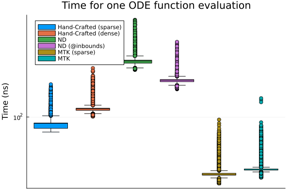
Benchmarks

Being able to easily define systems is well and good, but ultimately we also care about how fast the generated code is. For that purpose, I benchmarked the generated ODE functions for all three methods on a network with 5 nodes (see the notebook for details). In addition to the code shown in this post, I am comparing the hand-crafted function with a dense matrix in the parameters, the ModelingToolkit function without the symbolic array (referred to a “sparse” in the plots), and the NetworkDynamics functions using @propagate_inbounds (which they use in their examples). I’m running these benchmarks on a Laptop with an i7-1165G7 2.80GHz CPU, and 16GiB of RAM running Linux Mint 20.3. See the beginning of the post for the Julia/package versions.

As we can see on the plot, ModelingToolkit is by far the fastest, with the version without symbolic array a little bit ahead. The hand crafted functions come next, with the sparse version a little faster. NetworkDynamics is trailing behind, with the @propagate_inbounds version being appreciably faster.

Now, this one test is obviously not conclusive enough. In particular, we need to look at what happens with larger systems. In the next figure, I repeated the previous benchmarks for multiple network sizes, and I’m plotting the median execution times of the ODE functions as a function of the number of nodes. I’m using Watts-Strogatz networks, which are sparse, so we should expect a difference in the scaling of the various approaches.

As we can see, both hand-crafted variants are about even up until $N=50$ nodes, after which the dense matmul starts to fall behind. The ModelingToolkit version is the most performant for low values, but the naive version catches up with the hand-crafted functions at around $N=15$ nodes, and scales quadratically as one would expect, whereas the version without the symbolic array is the fastest until 200 nodes (I couldn’t get it to work beyond that). NetworkDynamics on the other hand is consistently slower than the hand-crafted function with sparse matmul by roughly half an order of magnitude, but otherwise scales similarly with the number of nodes (as one would expect).

Note that while ModelingToolkit generates the fastest functions, actually generating them takes a substantial time (about 20 seconds for 100 nodes, and 245 seconds for 200 nodes). It will also hog memory very quickly (the 200 nodes sparse version takes about 5.8 GiB!).

Based on these observations, I’d stick with the hand-crafted method for most problems, using sparse matrices for large networks to save on memory. It would be nice if I found a way to work with ModelingToolkit for this, as it has the great advantage of being able to generate ODE functions that can run in parallel or on GPUs, which the hand-crafted functions can’t as they are. As for NetworkDynamics, it doesn’t perform great here, but this is not really the kind of systems it’s intended for.

Conclusion

Let’s summarize what we discussed in this post.

• When hand-crafting ODE functions, @views is your friend. So is mul!. It can be difficult to get rid of all the allocations in some cases, though.
• ModelingToolkit is pretty good, but doesn’t seem to handle large matrices of parameters well. Maybe I’m using it wrong, so it seems worth experimenting with. When debugging, scalarize is your friend. Beware compilation times.
• NetworkDynamics adds a bit of boilerplate, for seemingly lackluster performance. Admittedly it’s designed with heterogeneous systems like power networks in mind, but it seems like ModelingToolkit could do that job better. It should be noted that comparing it to mul! is a bit unfair, as the latter is heavily optimized. I suspect the adequate use of a few macros could help here.

Over all, each of the approaches covered here has its strengths and weaknesses. I will very likely come back to this with a more comprehensive set of benchmarks, comparing the effects of various options and optimizations, as well as more than just the function evaluations.

Appendix

In the making of this post, I made a number of rookie mistakes. I list the biggest ones here for the record.

I initially made the mistake of putting my parameters in arrays instead of tuples. This can dramatically affect performance. Always use tuples.

Another mistake was running the first benchmark in a Jupyter notebook. For some reason, the results are slightly different there. In particular, the hand-crafted versions outperform ModelingToolkit (on my laptop). Be careful what environment you’re running your benchmarks on.

The difference between using Sparse and Dense matmuls is obviously highly dependent on the actual graph being used. A draft of this post used Erdos-Renyi graphs for the second benchmark, in which case both matmuls were about even as the Laplacian matrix wasn’t sparse enough.

As was pointed out by one of the NetworkDynamics.jl devs, ModelingToolkit also provides Jacobians, which gives it a big advantage over the two other approaches when actually solving the ODEs, which cannot be appreciated when only looking at the ODE function evaluations.

One thing I didn’t use here, but tried and failed to get working a while ago is using Split ODEs to separate between the local nonlinear dynamics and the linear coupling dynamics. I don’t expect this to affect the ODE function performance in this case.